Study for Voice and Emotion Detection

Glosary

Digital Signal Processing (DSP) = DSP is the use of digital processing to perform a wide variety of signal processing operations.
Waveform = A waveform describes a wave by graphing how an air molecule is displaced, over time.
Pulse-Code Modulation (PCM) = Pulse-code modulation (PCM) is a method used to represent sampled analog signals.
Frequency = Frequency is the measure of how many times the waveform repeats in a given amount of time.
Hertz (Hz) = The common unit of measurements for frequency. Hz represents the number the waveform repetitions per second.
Ampliture = A measure of how much a molecule is displaced from its resting position.
Sampling = In DSP, sampling is the reduction of continuous-time signal to a discrete-time signal.
Formant = A formant is a concentration of acoustic energy around a particular frequency in the speech wave.
Nyquist Theorem = The Nyquist Theorem states that in order to adequately reproduce a signal, it should be periodically sampled at a rate that is 2X the highest frequency you wish to record.
Windowing = Windowing is the process of taking a small subset of a larger dataset for processing or analysis.
Spectrogram = A spectrogram is a visual representation of a signal as it varies with time.
Fourier transform (FT) = FT is a mathematical transform which decomposes a function ( a signal) into its constituent frequencies.
Short-time Fourier transform (STFT) = STFT is a Fourier-related transform used to determine the sinusoidal frequency and phase content of local sections of a signal as it changes over time.
Voltage root-mean square (VRMS) = VRMS is defined as square root of the mean of the squares of the values for the one time period of the sine wave.

Helpful links

Waveform

Speech signals are sound signals, defined as pressure variations travelling through the air.

A speech signal is then represented by a sequence of numbers \(x_n\), which represent the relative air pressure at time-instant n∈ℕ.

This representation is known as pulse code modulation often abbreviated as PCM.

The accuracy of this representation is then specified by two factors;

the sampling frequency (the step in time between \(n\) and \(n+1\)).
the accuracy and distribution of amplitudes of \(x_n\) .

Sampling Rate

In DSP Sampling is the reduction of a continuous-time signal to a discrete-time signal.

A common example is the conversion of a sound wave (a continuous signal) to a sequence of samples (a discrete-time signal).

An important aspect of Sampling is the Nyquist Theorem. The Nyquist Theorem states that in order to adequately reproduce a continuous-time signal it should sampled at a rate that is 2X the highest frequency you wish to record.

Nyquist Sampling

\[(f) = d/2\]

Nyquist Sampling (f) = d, where d is the highest frequency you wish to record / 2

Most important information in speech signals are the formants, which reside in the range 300Hz - 3500Hz. This means that the lower limit of the sampling rate will have to be between 7-8kHz.

Windowing

A spoken sentence is a sequence of phonemes. Speech signals are therefore time-variant in character. To extract information from a speech signal, the signal must be split into sufficiently short segments, such that heuristically speaking, each segment contains only one phoneme.

Another way to think of this is to extract segments which are short enough that the properties of the speech signal does not have time to change within that segment.

Windowing a common method in signal processing. It is used to split the input signal into temporal segments. When windowing is applied to a signal the borders of the segment are visible as discontinuities.

In other words a windowed segment will have borders that go to zero. Windowing does change the signal however, the change is designed such that its effects on the signal are minimised.

There are two distinct applications of windowing with different requirements;

Analysis
Processing

In analysis the aim is to extract information as accurately as possible. In processing in addition to extracting information we also require the ability to recreate the signal from a sequence of windows.

A standard Hamming window is presented below.

import numpy as np
import matplotlib.pyplot as plt

window = np.hamming(51)
plt.plot(window)
plt.title("Hamming Window")
plt.ylabel("Ampliture")
plt.xlabel("Sample")

Text(0.5, 0, 'Sample')

png

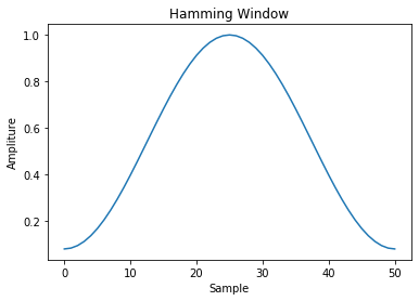
For signal analysis we would like the windowed signal to resemble the original signal as much as possible. When choosing a windowing function for analysis, the main criteria to consider is spectral distortion.

For signal processing the most common technique is to use a technique known as overlap-add.

png

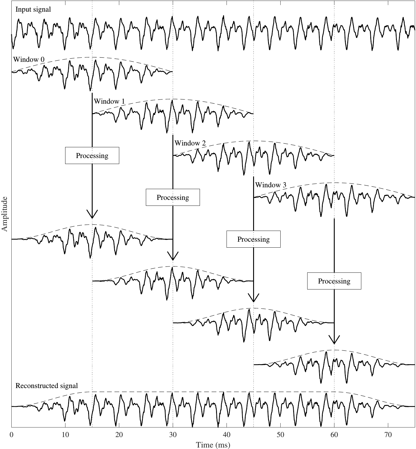
In overlap-add, we extract overlapping windows of the signal, apply some processing and reconstruct by windowing a second time and then adding overlapping segments together.

Spectrogram and Short-time Fourier transform (STFT)

The Fourier spectrum of a signal reveals the signals constituent frequencies. Revealing the Fourier spectrum of a signal is an intuitive way of examining the signal.

As mentioned earlier speech signals are non-stationary signals. Applying a Fourier transform or visualising the spectrogram of the entire signal will reveal the average of all phonemes in the sentence.

When the goal is to recognise each phoneme separately, we can focus on a single phonome at a time by applying a window to the signal. By windowing and applying a discrete fourier transformation on each window we obtain the Short-time Fourier transform.

# OS library
import os
from os.path import isdir, join
from pathlib import Path
import pandas as pd

# Math
import numpy as np
from scipy.fftpack import fft
from scipy import signal
from scipy.io import wavfile

from sklearn.decomposition import PCA

# Visualization
import matplotlib.pyplot as plt
import IPython.display as ipd


%matplotlib inline

Implementation of scipy.signal.stft and scipy.signal.spectrogram

Code taken from official scipy doc pages.

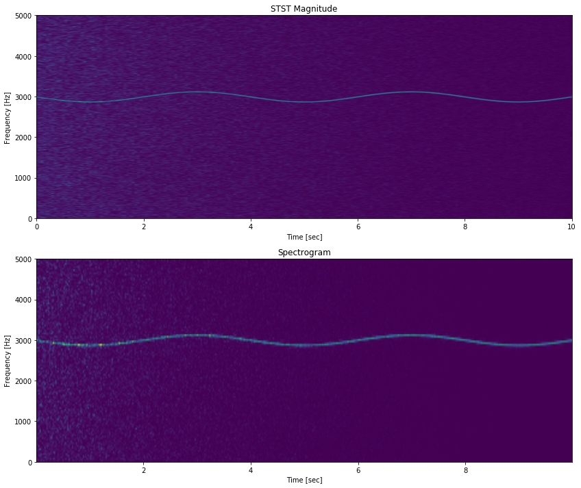
Generate a test signal, a 2 Vrms sine wave whose frequency is slowly modulated around 3kHz, corrupted by white noise of exponentially decreasing magnitude sampled at 10 kHz.

To break this down a little. What is Vrms. First, this is a really good reference page for this formula. http://www.referencedesigner.com/rfcal/cal_04.php

Vrms, Voltage root-mean square is defined as square root of the mean of the squares of the values for the one time period of the sine wave.

The formula can be used to the heating effect of a voltage in a resistor. In the code snipet below it is used to define the peaks of the sinusoids.

What is the difference between scipy.signal.stft and scipy.signal.spectrogram

The short-time Fourier transform (STFT), is a Fourier-related transform used to determine the sinusoidal frequency and phase content of local sections of a signal as it changes over time.

In practice, the procedure for computing STFTs is to divide a longer time signal into shorter segments of equal length and then compute the Fourier transform separately on each shorter segment.

This reveals the Fourier spectrum on each shorter segment. One then usually plots the changing spectra as a function of time.

A spectrogram is a visual representation of the spectrum of frequencies of a signal as it varies with time.

The spectrogram basically cuts your signal in small windows, and display a range of colors showing the intensity of this or that specific frequency. Exactly as the STFT. In fact it’s using the STFT.

By definition, the spectrogram is squared magnitude of the short-time Fourier transform (STFT) of the signal s(t):

spectrogram \((t, w) = [STFT(t, w)]^2\)

The stft function shows a linear visualisation because of the abs function whereas, spectrogram does not.

# Generating a test signal

# fs = sample rate
fs = 10e3

N = 1e5

# amp
amp = 2 * np.sqrt(2)

# noise power
noise_power = 0.01 * fs / 2

# time
time = np.arange(N) /float(fs)
mod = 500*np.cos(2*np.pi*0.25*time)
carrier = amp * np.sin(2*np.pi*3e3*time + mod)

# noise
noise = np.random.normal(scale=np.sqrt(noise_power),
                        size=time.shape)
noise *= np.exp(-time/5)
x = carrier + noise

# Visualisation
fig = plt.figure(figsize=(14, 12))

ax1 = fig.add_subplot(211)

f, t, Zxx = signal.stft(x, fs, nperseg=1000)
ax1.pcolormesh(t, f, np.abs(Zxx), vmin=0,
      vmax=amp, shading='gouraud')
ax1.set_title('STST Magnitude')
ax1.set_ylabel('Frequency [Hz]')
ax1.set_xlabel('Time [sec]')

ax2 = fig.add_subplot(212)

f, t, Sxx = signal.spectrogram(x, fs)
ax2.pcolormesh(t, f, Sxx, shading='gouraud')
ax2.set_title('Spectrogram')
ax2.set_ylabel('Frequency [Hz]')
ax2.set_xlabel('Time [sec]')
plt.show()

png

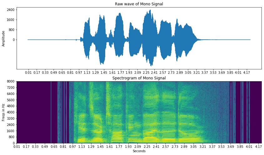
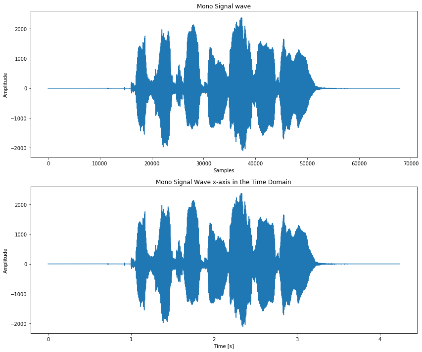
Analysis and visualisations on a Mono Sound file from the TIMIT dataset

# Standard way of reasing wav files with scypi
samplerate, samples = wavfile.read('output1.wav')

length = samples.shape[0] / samplerate
print(f"Signal length in seconds = {length}s")
print(f"Signal data type = {samples.dtype}")
print(f"Number of samples = {samples.shape[0]}")
print("Samplerate =", samplerate)

Signal length in seconds = 4.2375625s
Signal data type = int16
Number of samples = 67801
Samplerate = 16000

# Visualising Amplitude in the sample and time domains.

"""
Visualising a mono signal converted from stereo
using ffmpeg.

I have had trouble in the past reading in .wav
files and plotting any sort of visualisations due
to issues with mono/stereo. This can be remedied
but for simplicity I have converted the file using
the following snipet.

ffmpeg -i test.wav -acodec pcm_s16le
                    -ac 1 -ar 16000 output1.wav

"""

# Splicing for X to X seconds
#signal = signal[int(0.9 *
#sample_rate):int(3.3 * sample_rate)]

# Splicing for X to X samples
#signal = signal[int(5000):int(30000)]


"""
To Plot the x-axis in seconds you need get the
frame rate and divide by size of your signal.
linspace function from numpy is used to create
a Time Vector spaced linearly with the size of
the audio fileand finally you can use plot
again like plt.plot(Time,signal)

Time = np.linspace(0, len(signal)
                / 16000, num=len(signal))

"""

fig = plt.figure(figsize=(14, 12))

# First plot for Amplitude / Sample graph
ax1 = fig.add_subplot(211)
ax1.set_title("Mono Signal wave")
ax1.set_xlabel('Samples')
ax1.set_ylabel('Amplitude')
ax1.plot(signal)

# Second plot is Amplitude / Time graph
ax2 = fig.add_subplot(212)
ax2.set_title("Mono Signal Wave x-axis \
        in the Time Domain")
ax2.set_xlabel('Time [s]')
ax2.set_ylabel('Amplitude')
ax2.plot(np.linspace(0, len(signal) / sample_rate,
      num=len(signal)), signal)

plt.show()

png

Reading Stereo files with scipy

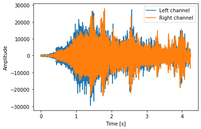
One of the first challenges I’ve had with reading .wav files is getting an error when reading stereo files with scipy.io.wavfile.read.

I’ve been able to work through this and found this very clear explanation on stackoverflow.

scipy.io.wavfile.read returns the tuple (rate, data). If the file is stereo, data is a numpy array with shape (nsamples, 2). To get a specific channel, use a slice of data.

rate, data = wavfile.read(path)
# data0 is the data from channel 0.
data0 = data[:, 0]

# Reading in a new .wav file
sample_rate, signal = wavfile.read('test.wav')

# Splicing the signal for 0 to 3.3 secs
signal = signal[0:int(3.3 * sample_rate)]

# Using np.linspace to create evenly space
# sequence of samples.
# np.linspace(start = , stop= , number of
# items to generate within the range= )
# in this case starts at 0s, stops at 4.2375625s,
# generates 67801 items.
time = np.linspace(0., samples.shape[0] /
            \ samplerate, signal.shape[0])

# plots time variable in x axis and left
# channel amplitude on y axis
plt.plot(time, signal[:, 0], label="Left channel")
# plots time variable in x axis and right channel
# amplitude on y axis
plt.plot(time, signal[:, 1], label="Right channel")
plt.legend()
plt.xlabel("Time [s]")
plt.ylabel("Amplitude")
plt.show()

png

sample_rate, samples =
              scipy.io.wavfile.read('output1.wav')


def log_specgram(audio, sample_rate, window_size=20,
                 step_size=10, eps=1e-10):
    nperseg = int(round(window_size * sample_rate / 1e3))
    noverlap = int(round(step_size * sample_rate / 1e3))
    freqs, times, spec = signal.spectrogram(audio,
                                    fs=sample_rate,
                                    window='hann',
                                    nperseg=nperseg,
                                    noverlap=noverlap,
                                    detrend=False)
    return freqs, times, \
          np.log(spec.T.astype(np.float32) + eps)


freqs, times, spectrogram =
                    log_specgram(samples, sample_rate)

fig = plt.figure(figsize=(14, 8))
ax1 = fig.add_subplot(211)
ax1.set_yticks(freqs[::16])
ax1.set_xticks(times[::16])
ax1.set_title('Raw wave of Mono Signal')
ax1.set_ylabel('Amplitude')
ax1.plot(np.linspace(0, len(samples) /
              sample_rate, num=len(samples)), samples)

ax2 = fig.add_subplot(212)
ax2.imshow(spectrogram.T,
            aspect='auto',
            origin='lower',
          extent=[times.min(),
          times.max(),
          freqs.min(),
          freqs.max()])
ax2.set_yticks(freqs[::16])
ax2.set_xticks(times[::16])
ax2.set_title('Spectrogram of Mono Signal')
ax2.set_ylabel('Freqs in Hz')
ax2.set_xlabel('Seconds')

Text(0.5, 0, 'Seconds')

png